Something I recently became interested in is map data structures for external memory — i.e. ways of storing indexed data that are optimized for storage on disk.

In a typical analysis of algorithm time complexity, you assume it takes constant time to access memory or perform a basic CPU operation such as addition. This is of course not wholly accurate: in particular, cache effects mean that memory access time varies wildly depending on what exact address you are querying. In a system where your algorithm may access external memory, this becomes even more true — a CPU that takes 1ns to perform an addition may easily find itself waiting 5ms (i.e. 5 million ns) for a read from a spinning disk to complete.

An alternative model of complexity is the Disk Access Machine (DAM). In this model, reading one block of memory (of fixed size B) has constant time cost, and all other operations are free. Just like its conventional cousin this is clearly a simplification of reality, but it's one that lets us succinctly quantify the disk usage of various data structures.

At the time of writing, this is the performance we can expect from the storage hierarchy:

Category	Representative device	Sequential Read Bandwidth	Sequential Write Bandwidth	4KB Read IOPS	4KB Write IOPS
Mechanical disk	Western Digital Black WD4001FAEX (4TB)	130MB/s	130MB/s	110	150
SATA-attached SSD	Samsung 850 Pro (1TB)	550MB/s	520MB/s	10,000	36,000
PCIe-attached SSD	Intel 750 (1.2TB)	2,400MB/s	1,200MB/s	440,000	290,000
Main memory	Skylake @ 3200MHz	42,000MB/s	48,000MB/s	16,100,000 (62ns/operation)

(In the above table, all IOPS figures are reported assuming a queue depth of 1, so will tend to be worst case numbers for the SSDs.)

Observe that the implied bandwidth of random reads from a mechanical disk is (110 * 4KB/s) i.e. 440KB/s — approximately 300 times slower than the sequential read case. In contrast, random read bandwith from a PCIe-attached SSD is (440,000 * 4KB/s) = 1.76GB/s i.e. only about 1.4 times slower than the sequential case. So you still pay a penalty for random access even on SSDs, but it's much lower than the equivalent cost on spinning disks.

One way to think about the IOPS numbers above is to break them down into that part of the IOPS that we can attribute to the time necessary to transfer the 4KB block (i.e. 4KB/Bandwidth) and whatever is left, which we can call the seek time (i.e. (1/IOPS) - (4KB/Bandwidth)):

Category	Implied Seek Time From Read	Implied Seek Time From Write	Mean Implied Seek Time
Mechanical Disk	9.06ms	6.63ms	7.85ms
SATA-attached SSD	92.8us	20.2us	56.5us
PCIe-attached SSD	645ns	193ns	419ns

If we are using the DAM to model programs running on top of one of these storage mechanisms, which block size B should we choose such that algorithm costs derived from the DAM are a good guide to real-world time costs? Let's say that our DAM cost for some algorithm is N block reads. Consider two scenarios:

• If these reads are all contiguous, then the true time cost (in seconds) of the reads will be N*(B/Bandwidth) + Seek Time
• If they are all random, then the true time cost is N*((B/Bandwidth) + Seek Time), i.e. (N - 1)*Seek Time more than the sequential case

The fact that the same DAM cost can correspond to two very different true time costs suggests that in we should try to choose a block size that minimises the difference between the two possible true costs. With this in mind, a sensible choice is to set B equal to the product of the seek time and the bandwidth of the device. If we do this, then in random-access scenario (where the DAM most underestimates the cost):

• Realized IOPS will be at least half of peak IOPS for the storage device.
• Realized bandwidth will be at least half of peak bandwidth for the storage device.

If we choose B smaller than the bandwidth/seek time product then we'll get IOPS closer to device maximum, but only at the cost of worse bandwidth. Likewise, larger blocks than this will reduce IOPS but boost bandwidth. The proposed choice of B penalises both IOPS and bandwidth equally. Applying this idea to the storage devices above:

Category	Implied Block Size From Read	Implied Block Size From Write	Mean Implied Block Size
Mechanical Disk	1210KB	883KB	1040KB
SATA-attached SSD	52.3KB	10.8KB	31.6KB
PCIe-attached SSD	1.59KB	243B	933B

On SSDs the smallest writable/readable unit of storage is the page. On current generation devices, a page tends to be around 8KB in size. It's gratifying to see that this is within an order of magnitude of our SSD block size estimates here.

Interestingly, the suggested block sizes for mechanical disks are much larger than the typical block sizes used in operating systems and databases, where 4KB virtual memory/database pages are common (and certainly much larger than the 512B sector size of most spinning disks). I am of course not the first to observe that typical database page sizes appear to be far too small.

Applying the DAM

Now we've decided how we can apply the DAM to estimate disk costs that will translate (at least roughly) to real-world costs, we can actually apply the model to the analysis of some algorithms. Before we begin, some interesting features of the DAM:

• Binary search is not optimal. Binary-searching N items takes O(log (N/B)) block reads, but O(log_B N) search is possible with other algorithms.
• Sorting by inserting items one at a time into a B-tree and then traversing the tree is not optimal. The proposed approach takes O(N log_B N) but it's possible to sort in O((N/B) * log (N/B)).
• Unlike with the standard cost model, many map data structures have different costs for lookup and insertion in the DAM, which means that e.g. adding UNIQUE constraints to database indexes can actually change the complexity of inserting into the index (since you have to do lookup in such an index before you know whether an insert should succeed).

Now let's cover a few map data structures. We'll see that the maps that do well in the DAM model will be those that are best able to sequentialize their access patterns to exploit the block structure of memory.

2-3 Tree

The 2-3 tree is a balanced tree structure where every leaf node is at the same depth, and all internal nodes have either 1 or 2 keys — and therefore have either 2 or 3 children. Leaf nodes have either 1 or 2 key/value pairs.

Lookup in this tree is entirely straightforward and has complexity O(log N). Insertion into the tree proceeds recursively starting from the root node:

1. If inserting into a leaf, we add the data item to the leaf. Note that this may mean that the leaf temporarily contain 3 key/value pairs, which is more than the usual limit.
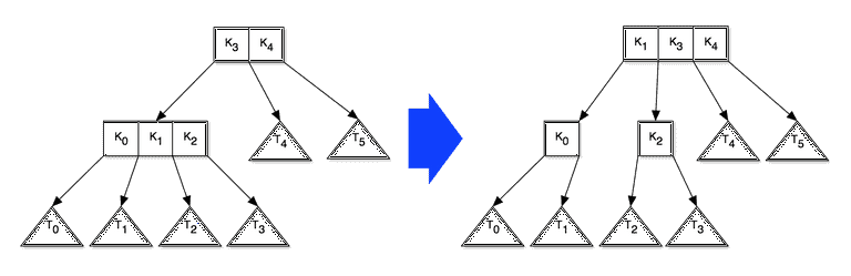
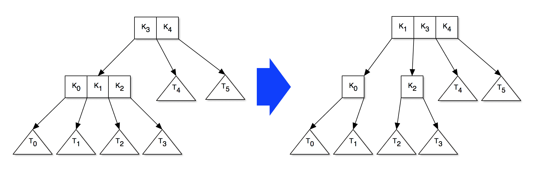
2. If inserting into a internal node, we recursively add the data item to the appropriate child. After doing this, the child may contain 3 keys, in which case we pull one up to this node, creating a new sibling in the process. If this node already contained 2 keys this will in turn cause it to become oversized. An example of how this might look is:
   
   
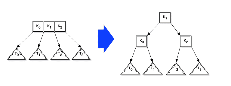
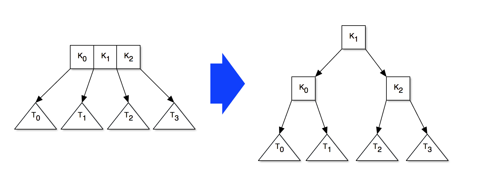
3. If, after the recursion completes, the root node contains 3 keys, then we pull a new root node (with one key) out of the old root, like so:
   
   

It's easy to see that this keeps the tree balanced. This insertion process also clearly has O(log N) time complexity, just like lookup. The data structure makes no attempt to exploit the fact that memory is block structured, so both insertion and lookup have identical complexity in the DAM and the standard cost model.

B-Tree

The B-tree (and the very closely related B+tree) is probably the most popular structure for external memory storage. It can be seen as a simple generalisation of the 2-3 tree where, instead of each internal node having 1 or 2 keys, it instead has between m and 2m keys for any m > 0. We then set m to the maximum value so that one internal node fits exactly within our block size B, i.e. m = O(B).

In the DAM cost model, lookup in a B-tree has time complexity O(log_B N). This is because we can access each internal node's set of at least m keys using a single block read — i.e. in O(1) — and this lets us make a choice between at least m+1 = O(B) child nodes.

For similar reasons to the lookup case, inserting into a B-tree also has time cost O(log_B N) in the DAM.

Buffered Repository Tree

A buffered repository tree, or BRT, is a generalization of a 2-3 tree where each internal node is associated with an additional buffer of size k = O(B). When choosing k a sensible choice is to make it just large enough to use all the space within a block that is not occupied by the keys of the internal node.

When inserting into this tree, we do not actually modify the tree structure immediately. Instead, a record of the insert just gets appended to the root node's buffer until that buffer becomes full. Once it is full, we're sure to be able to spill at least k/3 insertions to one child node. These inserts will be buffered at the lower level in turn, and may trigger recursive spills to yet-deeper levels.

What is the time complexity of insertion? Some insertions will be very fast because they just append to the buffer, while others will involve extensive spilling. To smooth over these differences, we therefore consider the amortized cost of an insertion. If we insert N elements into the tree, then at each of the O(log (N/B)) levels of the tree we'll spill at most O(N/(k/3)) = O(N/B) times. This gives a total cost for the insertions of O((N/B) log (N/B)), which is an amortized cost of O((log (N/B))/B).

Lookup proceeds pretty much as normal, except that the buffer at each level must be searched before any child nodes are considered. In the DAM, this additional search has cost O(1), so lookup cost becomes O(log (N/B)).

Essentially what we've done with this structure is greatly sped up the insertion rate by exploiting the fact that the DAM lets us batch up writes into groups of size O(B) for free. This is our first example of a structure whose insertion cost is lower than its lookup cost.

B-ε Tree

It turns out that it's possible to see the B-tree and the BRT as the two most extreme examples of a whole family of data structures. Specifically, both the B-tree and the BRT are instances of a more general notion called a B-ε tree, where ε is a real variable ranging between 0 and 1.

A B-ε tree is a generalisation of a 2-3 tree where each internal node has between m and 2m keys, where 0 < m = O(B^ε). Each node is also accompanied by a buffer of size k = O(B). This buffer space is used to queue pending inserts, just like in the BRT.

One possible implementation strategy is to set m so that one block is entirely full with keys when ε = 1, and so that m = 2 when ε = 0. The k value can then be chosen to exactly occupy any space within the block that is not being used for keys (so in particular, if ε = 1 then k = 0). With these definitions it's clear that the ε = 1 case corresponds to a B-tree and ε = 0 gives you a BRT.

As you would expect, the B-ε insertion algorithm operates in essentially the same manner as described above for the BRT. To derive the time complexity of insertion, we once again look at the amortized cost. Observe that the structure will have O(log_B^ε (N/B)) = O((log_B (N/B))/ε) = O((log_B N)/ε) levels and that on each spill we'll be able to push down at least O(B^1-ε) elements to a child. This means that after inserting N elements into the tree, we'll spill at most O(N/(B^1-ε)) = O(N*B^ε-1) times. This gives a total cost for the insertions of O(N*B^ε-1*(log_B N)/ε), which is an amortized cost of O((B^ε-1/ε)*log_B N).

The time complexity of lookups is just the number of levels in the tree i.e. O((log_B N)/ε).

Fractal Tree

These complexity results for the B-ε tree suggest a tantalising possibility: if we set ε = ½ we'll have a data structure whose asymptotic insert time will be strictly better (by a factor of sqrt B) than that of B-trees, but which have exactly the same asymptotic lookup time. This data structure is given the exotic name of a "fractal tree". Unfortunately, the idea is patented by the founders of Tokutek (now Percona), so they're only used commercially in Percona products like TokuDB. If you want to read more about what you are missing out on, there's a good article on the company blog and a whitepaper.

Log-Structured Merge Tree

The final data structure we'll consider, the log-structured merge tree (LSMT) rivals the popularity of the venerable B-tree and is the technology underlying most "NoSQL" stores.

In a LSMT, you maintain your data in a list of B-trees of varying sizes. Lookups are accomplished by checking each B-tree in turn. To avoid lookups having to check too many B-trees, we arrange that we never have too many small B-trees in the collection.

There are two classes of LSMT that fit this general scheme: size-tiered and levelled.

In a levelled LSMT, your collection is a list of B-trees of size at most O(B), O(B*k), O(B*k²), O(B*k³), etc for some growth factor k. Call these level 0, 1, 2 and so on. New items are inserted into level 0 tree. When this tree exceeds its size bound, it is merged into the level 1 tree, which may trigger recursive merges in turn.

Observe that if we insert N items into a levelled LSMT, there will be O(log_k (N/B)) B-trees and the last one will have O(N/B) items in it. Therefore lookup has complexity O(log_B N * log_k (N/B)). To derive the update cost, observe that the items in the last level have been merged down the full O(log_k (N/B)) levels, and they will have been merged into on average O(k) times in each level before moving down to the next. Therefore the amortized insertion cost is O((k * log_k (N/B)) / B).

If we set k = ½ then lookup and insert complexity simplify to O((log_B N)²) and O(log_B N / sqrt B) respectively.

In a size-tiered LSMT things are slightly different. In this scheme we have a staging buffer of size O(B) and more than one tree at each level: specifically, at level i >= 0, we have up to k B-trees of size exactly O(B*kⁱ). New items are inserted inte the staging buffer. When it runs out of space, we turn it into a B-tree and insert it into level 0. If would causes us to have more than k trees in the level, we merge the k trees together into one tree of size O(B*k) that we can try to insert into level 1, which may in turn trigger recursive merges.

The complexity arguments we made for levelled LSMT carry over almost unchanged into this new setting, showing that the two schemes have identical costs. LSMTs match the insert performance of fractal trees, but suffer the cost of an extra log factor when doing lookup. To try to improve lookup time, in practice most LSMT implementations store each B-tree along with a Bloom filter which allows them to avoid accessing a tree entirely when a key of interest is certainly not included in it.

There are several good overviews of LSMTs available online.

Experiments

To validate my knowledge of these data structures, I wrote a Python program that tries to perform an apples-to-apples comparison of various B-ε tree variants. The code implements the datastructure and also logs how many logical blocks it would need to touch if the tree was actually implemented on a block-structured device (in reality I just represent it as a Python object). I assume that as many of the trees towards the top of the tree as possible are stored in memory and so don't hit the block device.

I simulate a machine with 1MB of memory and 32KB pages. Keys are assumed to be 16 bytes and values 240 bytes. With these assumptions can see how the number of block device pages we need to write to varies with the number of keys in the tree for each data structure:

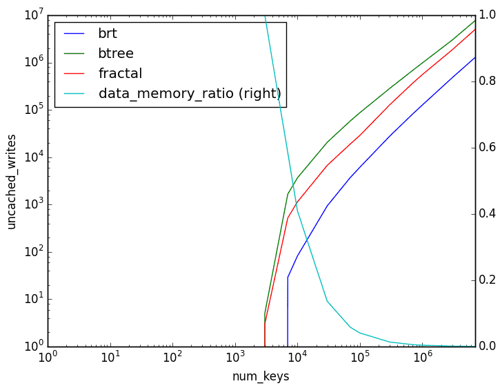
These experimental results match what we would expect from the theoretical analysis: the BRT has a considerable advantage over the alternatives when it comes to writes, B-trees are the worst, and fractal trees occupy the middle ground.

The equivalent results for reads are as follows:

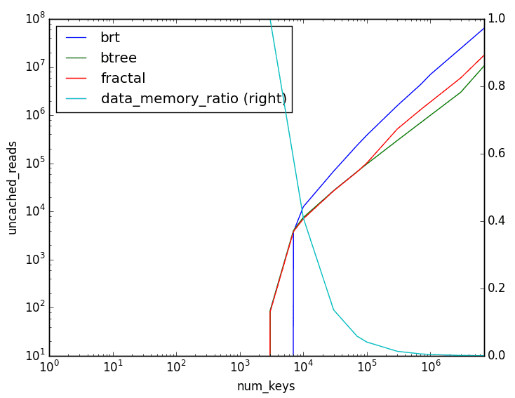
This is essentially a mirror image of the write results, showing that we're fundamentally making a trade-off here.

Summary

We can condense everything we've learnt above into the following table:

Structure	Lookup	Insert
2-3 Tree	O(log N)	O(log N)
B-ε Tree	O((logB N)/ε)	O((Bε-1/ε)*logB N)
B-Tree (ε=1)	O(logB N)	O(logB N)
Fractal Tree (ε=½)	O(logB N)	O(logB N / sqrt B)
Buffered Repository Tree (ε=0)	O(log (N/B))	O((log (N/B))/B)
Log Structured Merge Tree	O((logB N)2)	O(logB N / sqrt B)

These results suggest that you should always prefer to use a fractal tree to any of a B-tree, LSMT or 2-3 tree. In the real world, things may not be so clear cut: in particular, because of the fractal tree patent situation, it may be difficult to find a free and high-quality implementation of that data structure.

Most engineering effort nowadays is being directed at improving implementations of B-trees and LSMTs, so you probably want to choose one of these two options depending on whether your workload is read or write heavy, respectively. Some would argue, however, that all database workloads are essentially write bound, given that you can usually optimize a slow read workload by simply adding some additional indexes.